Use a discrete likelihood

import tensorflow_probability as tfp
import tensorflow as tf
import numpy as np
import elicit as el

tfd = tfp.distributions

Use a discrete likelihood#

Gradients for discrete RVs#

Challenge#

ToDo (describe the problem of computing gradients for discrete RVs)
possible solution: softmax-gumble trick

Possible work around: Softmax-Gumble Trick#

Describe the softmax gumble trick

Example: Binomial model#

\[\begin{align*} \beta_0 &\sim \text{Normal}(\mu_0, \sigma_0) &\text{priors}\\ \beta_1 &\sim \text{Normal}(\mu_1, \sigma_1) &\\ \mu &= \text{sigmoid}(\beta_0 + \beta_1X) &\text{link+linear predictor} \\ y_i &\sim \text{Binomial}(\mu, N) &\text{likelihood} \end{align*}\]

using the el.utils.softmax_gumble_trick() function in the generative model

help(el.utils.softmax_gumbel_trick)

Help on function softmax_gumbel_trick in module elicit.utils:

softmax_gumbel_trick(epred: tensorflow.python.framework.tensor.Tensor, likelihood: <built-in function callable>, upper_thres: float, temp: float = 1.6, **kwargs)
    The softmax-gumbel trick computes a continuous approximation of ypred from
    a discrete likelihood and thus allows for the computation of gradients for
    discrete random variables.
    
    Currently this approach is only implemented for models without upper
    boundary (e.g., Poisson model).
    
    Corresponding literature:
    
    - Maddison, C. J., Mnih, A. & Teh, Y. W. The concrete distribution:
        A continuous relaxation of
      discrete random variables in International Conference on Learning
      Representations (2017). https://doi.org/10.48550/arXiv.1611.00712
    - Jang, E., Gu, S. & Poole, B. Categorical reparameterization with
    gumbel-softmax in International Conference on Learning Representations
    (2017). https://openreview.net/forum?id=rkE3y85ee.
    - Joo, W., Kim, D., Shin, S. & Moon, I.-C. Generalized gumbel-softmax
    gradient estimator for generic discrete random variables.
      Preprint at https://doi.org/10.48550/arXiv.2003.01847 (2020).
    
    Parameters
    ----------
    epred : tf.Tensor
        simulated linear predictor from the model simulations 
    likelihood : tfp.distributions object, shape = [B, num_samples, num_obs, 1]
        likelihood function used in the generative model.
        Must be a tfp.distributions object.
    upper_thres : float
        upper threshold at which the distribution of the outcome variable is
        truncated. For double-bounded distribution (e.g. Binomial) this is
        simply the "total count" information. Lower-bounded distribution
        (e.g. Poisson) must be truncated to create an artificial
        double-boundedness.
    temp : float, temp > 0
        temperature hyperparameter of softmax function. A temperature going
        towards zero yields approximates a categorical distribution, while
        a temperature >> 0 approximates a continuous distribution.
        The default value is ``1.6``.
    kwargs : any
        additional keyword arguments including the seed information. **Note**:
        the ``**kwargs`` argument is required in this function (!) as it
        extracts internally the seed information.
    
    Returns
    -------
    ypred : tf.Tensor
        continuously approximated ypred from the discrete likelihood.
    
    Raise
    -----
    ValueError
        if rank of ``likelihood`` is not 4. The shape of the likelihood obj
        must have an extra final dimension, i.e., (B, num_samples, num_obs, 1),
        for the softmax-gumbel computation. Use for example
        ``tf.expand_dims(mu,-1)`` for expanding the batch-shape of the
        likelihood.
    
        if likelihood is not in tfp.distributions module. The likelihood
        must be a tfp.distributions object.
    
    KeyError
        if ``**kwargs`` is not in function arguments. It is required to pass
        the **kwargs argument as it is used for extracting internally 
        information about the seed.

The generative model#

class ToyModel:
    def __call__(self, prior_samples, design_matrix, total_count, temp,
                 **kwargs):
        B = prior_samples.shape[0]
        S = prior_samples.shape[1]

        # preprocess shape of design matrix
        X = tf.broadcast_to(design_matrix[None, None,:],
                           (B,S,len(design_matrix)))
        # linear predictor (= mu)
        epred = tf.add(prior_samples[:, :, 0][:,:,None],
                       tf.multiply(prior_samples[:, :, 1][:,:,None], X)
                       )
        # data-generating model
        likelihood = tfd.Binomial(
            total_count=total_count,
            probs=tf.math.sigmoid(tf.expand_dims(epred,-1)))

        # prior predictive distribution 
        ypred = el.utils.softmax_gumbel_trick(
            likelihood, total_count, temp, **kwargs)
        
        # selected observations
        y_X0, y_X1, y_X2 = (ypred[:,:,0], ypred[:,:,1], ypred[:,:,2])

        return dict(y_X0=y_X0, y_X1=y_X1, y_X2=y_X2)

Construct the predictor#

# numeric, standardized predictor
def std_predictor(N, quantiles):
    X = tf.cast(np.arange(N), tf.float32)
    X_std = (X-tf.reduce_mean(X))/tf.math.reduce_std(X)
    X_sel = tfp.stats.percentile(X_std, [int(p*100) for p in quantiles])
    return X_sel

design_matrix = std_predictor(N=200, quantiles=[0.25, 0.50, 0.75])
design_matrix.numpy()

array([-0.85737586,  0.00866036,  0.85737586], dtype=float32)

Oracle as expert#

we simulate from a ground truth to obtain the expert data

\[\begin{align*} \beta_0 &\sim \text{Normal}(0.1, 0.4)\\ \beta_1 &\sim \text{Normal}(0.2, 0.2) \end{align*}\]

ground_truth = {
    "beta0": tfd.Normal(loc=0.1, scale=0.4),
    "beta1": tfd.Normal(loc=0.2, scale=0.2),
}

Parametric approach#

Specify the `eliobj`#

eliobj = el.Elicit(
    model=el.model(
        obj=ToyModel,
        design_matrix=design_matrix,
        total_count = 30,
        temp = 1.6
        ),
    parameters=[
        el.parameter(
            name="beta0",
            family=tfd.Normal,
            hyperparams=dict(
                loc=el.hyper("mu0"),
                scale=el.hyper("sigma0", lower=0)
                )
        ),
        el.parameter(
            name="beta1",
            family=tfd.Normal,
            hyperparams=dict(
                loc=el.hyper("mu1"),
                scale=el.hyper("sigma1", lower=0)
                )
        )
    ],
    targets=[
        el.target(
            name=f"y_X{i}",
            query=el.queries.quantiles((.05, .25, .50, .75, .95)),
            loss=el.losses.MMD2(kernel="energy"),
            weight=1.0
        ) for i in range(3)
    ],
    expert=el.expert.simulator(
        ground_truth = ground_truth,
        num_samples = 10_000
    ),
    optimizer=el.optimizer(
        optimizer=tf.keras.optimizers.Adam,
        learning_rate=0.05,
        clipnorm=1.0
        ),
    trainer=el.trainer(
        method="parametric_prior",
        seed=0,
        epochs=300
    ),
    initializer=el.initializer(
        method="sobol",
        loss_quantile=0,
        iterations=32,
        distribution=el.initialization.uniform(
            radius=1.,
            mean=0.
            )
    )
)

Train the `eliobj`#

eliobj.fit()

Initialization

100%|██████████| 32/32 [00:11<00:00,  2.69it/s]

 
Training

100%|██████████| 300/300 [02:56<00:00,  1.70it/s]

Results#

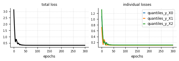
Convergence - Loss#

el.plots.loss(eliobj, figsize=(6,2))

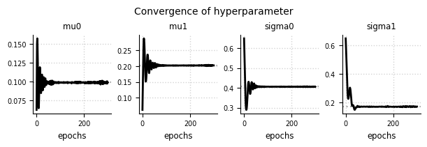
../_images/67f75b74355f512ae2815e2c2f0e272542f081ecb41abff59b8889734e3d48fd.png

Convergence - Hyperparameter#

el.plots.hyperparameter(eliobj, figsize=(6,2))

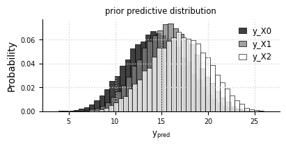
../_images/9be97c69b3aeb97d553ad9877b2e9e5d46ada38f6da8eef69c3487f9cbd467b2.png

Prior predictive distribution#

el.plots.priorpredictive(eliobj, figsize=(4,2))

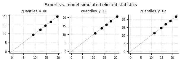
../_images/f78f8f3d0465dbee927988913ab2465144f1364cfa35f5dccbb4c8d2f3278735.png

Expert data (oracle) vs. simulated data#

el.plots.elicits(eliobj, cols=3, figsize=(6,2))

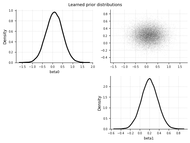
../_images/72cab7980bb561cf4a5f6ffddad819a2c972a0f7618ceda6296c99674e2978c3.png

Learned prior distributions#

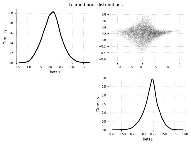
el.plots.priors(eliobj)

../_images/cfe89d7bbaa569eb30329e5a0d8e6fdba1f4276a6364c134c02ac432c0842f9c.png

Non-parametric approach#

Specify the `eliobj`#

from bayesflow.inference_networks import InvertibleNetwork

eliobj2 = el.Elicit(
    model=el.model(
        obj=ToyModel,
        design_matrix=design_matrix,
        total_count = 30,
        temp = 1.6
        ),
    parameters=[
        el.parameter(name="beta0"),
        el.parameter(name="beta1")
    ],
    targets=[
        el.target(
            name="y_X0",
            query=el.queries.quantiles((.05, .25, .50, .75, .95)),
            loss=el.losses.MMD2(kernel="energy"),
            weight=1.0
        ),
        el.target(
            name="y_X1",
            query=el.queries.quantiles((.05, .25, .50, .75, .95)),
            loss=el.losses.MMD2(kernel="energy"),
            weight=1.0
        ),
        el.target(
            name="y_X2",
            query=el.queries.quantiles((.05, .25, .50, .75, .95)),
            loss=el.losses.MMD2(kernel="energy"),
            weight=1.0
        )
    ],
    expert=el.expert.simulator(
        ground_truth = ground_truth,
        num_samples = 10_000
    ),
    optimizer=el.optimizer(
        optimizer=tf.keras.optimizers.Adam,
        learning_rate=0.001,
        clipnorm=1.0
        ),
    trainer=el.trainer(
        method="deep_prior",
        seed=0,
        epochs=200
    ),
    network=el.networks.NF(
        inference_network=InvertibleNetwork,
        network_specs=dict(
            num_params=2,
            num_coupling_layers=3,
            coupling_design="affine",
            coupling_settings={
                "dropout": False,
                "dense_args": {
                    "units": 128,
                    "activation": "relu",
                    "kernel_regularizer": None,
                },
                "num_dense": 2,
            },
            permutation="fixed"
        ),
        base_distribution=el.networks.base_normal
    )
)

Train the `eliobj`#

eliobj2.fit()

Training

100%|██████████| 200/200 [05:31<00:00,  1.66s/it]

Results#

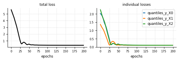
Convergence - Loss#

el.plots.loss(eliobj2, figsize=(6,2))

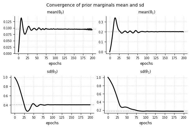
../_images/500e00e7cb8e7c83dc06639ac0571563aeb63d45d27a623233ffbdc1fd04b488.png

Convergence - Marginals#

el.plots.marginals(eliobj2, cols=2, figsize=(6,4))

../_images/fe26f01555e499d081a8675809938860e2f1fdde99e53f55947f4638214ff458.png

Prior predictive distribution#

el.plots.priorpredictive(eliobj2, figsize=(4,2))

---------------------------------------------------------------------------
KeyError                                  Traceback (most recent call last)
Cell In[27], line 1
----> 1 el.plots.priorpredictive(eliobj2, figsize=(4,2))

File ~\Documents\GitHub\prior_elicitation\elicit\plots.py:706, in priorpredictive(eliobj, **kwargs)
    704 B=eliobj.trainer["B"]
    705 num_samples=eliobj.trainer["num_samples"]
--> 706 n_obs = eliobj.results["model_samples"]["ypred"].shape[-1]
    708 pp_samples = tf.reshape(eliobj.results["model_samples"]["ypred"],
    709                         (B*num_samples,n_obs))
    712 fig, axs = plt.subplots(1, 1, constrained_layout=True, **kwargs)

KeyError: 'ypred'

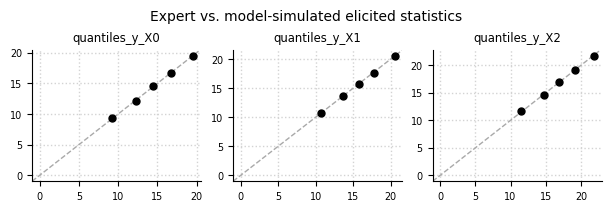
Expert data (oracle) vs. simulated data#

el.plots.elicits(eliobj2, cols=3, figsize=(6,2))

../_images/4a26470ea05945ab9820eef2cf0840ccd369f10588b4c474e196047682f5aa34.png

Learned prior distributions#

el.plots.priors(eliobj2)

../_images/662c3b52c5eecdd7d4c5f1dbfb229eaa7f9287f3809a1fa555c5f423dfe422f5.png

Use a discrete likelihood

Contents

Use a discrete likelihood#

Gradients for discrete RVs#

Challenge#

Possible work around: Softmax-Gumble Trick#

Example: Binomial model#

The generative model#

Construct the predictor#

Oracle as expert#

Parametric approach#

Specify the eliobj#

Train the eliobj#

Results#

Convergence - Loss#

Convergence - Hyperparameter#

Prior predictive distribution#

Expert data (oracle) vs. simulated data#

Learned prior distributions#

Non-parametric approach#

Specify the eliobj#

Train the eliobj#

Results#

Convergence - Loss#

Convergence - Marginals#

Prior predictive distribution#

Expert data (oracle) vs. simulated data#

Learned prior distributions#

Specify the `eliobj`#

Train the `eliobj`#

Specify the `eliobj`#

Train the `eliobj`#